Distributed Training · Apache SINGA

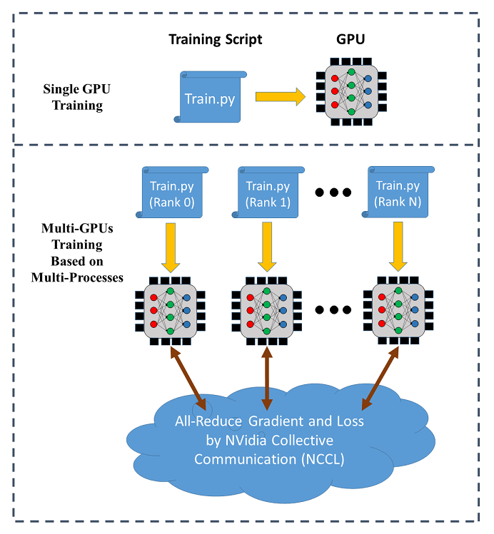
SINGA supports data parallel training across multiple GPUs (on a single node or across different nodes). The following figure illustrates the data parallel training:

In distributed training, each process (called a worker) runs a training script over a single GPU. Each process has an individual communication rank. The training data is partitioned among the workers and the model is replicated on every worker. In each iteration, the workers read a mini-batch of data (e.g., 256 images) from its partition and run the BackPropagation algorithm to compute the gradients of the weights, which are averaged via all-reduce (provided by NCCL) for weight update following stochastic gradient descent algorithms (SGD).

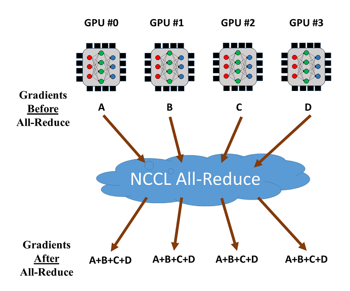
The all-reduce operation by NCCL can be used to reduce and synchronize the gradients from different GPUs. Let's consider the training with 4 GPUs as shown below. Once the gradients from the 4 GPUs are calculated, all-reduce will return the sum of the gradients over the GPUs and make it available on every GPU. Then the averaged gradients can be easily calculated.

Usage

SINGA implements a module called DistOpt (a subclass of Opt) for distributed training. It wraps a normal SGD optimizer and calls Communicator for gradients synchronization. The following example illustrates the usage of DistOpt for training a CNN model over the MNIST dataset. The source code is available here, and there is a Colab notebook for it.

Example Code

Define the neural network model:

class CNN(model.Model):

    def __init__(self, num_classes=10, num_channels=1):
        super(CNN, self).__init__()
        self.conv1 = layer.Conv2d(num_channels, 20, 5, padding=0, activation="RELU")
        self.conv2 = layer.Conv2d(20, 50, 5, padding=0, activation="RELU")
        self.linear1 = layer.Linear(500)
        self.linear2 = layer.Linear(num_classes)
        self.pooling1 = layer.MaxPool2d(2, 2, padding=0)
        self.pooling2 = layer.MaxPool2d(2, 2, padding=0)
        self.relu = layer.ReLU()
        self.flatten = layer.Flatten()
        self.softmax_cross_entropy = layer.SoftMaxCrossEntropy()

    def forward(self, x):
        y = self.conv1(x)
        y = self.pooling1(y)
        y = self.conv2(y)
        y = self.pooling2(y)
        y = self.flatten(y)
        y = self.linear1(y)
        y = self.relu(y)
        y = self.linear2(y)
        return y

    def train_one_batch(self, x, y, dist_option='fp32', spars=0):
        out = self.forward(x)
        loss = self.softmax_cross_entropy(out, y)

        # Allow different options for distributed training
        # See the section "Optimizations for Distributed Training"
        if dist_option == 'fp32':
            self.optimizer(loss)
        elif dist_option == 'fp16':
            self.optimizer.backward_and_update_half(loss)
        elif dist_option == 'partialUpdate':
            self.optimizer.backward_and_partial_update(loss)
        elif dist_option == 'sparseTopK':
            self.optimizer.backward_and_sparse_update(loss,
                                                      topK=True,
                                                      spars=spars)
        elif dist_option == 'sparseThreshold':
            self.optimizer.backward_and_sparse_update(loss,
                                                      topK=False,
                                                      spars=spars)
        return out, loss

# create model
model = CNN()

Create the DistOpt instance and attach it to the created model:

sgd = opt.SGD(lr=0.005, momentum=0.9, weight_decay=1e-5)
sgd = opt.DistOpt(sgd)
model.set_optimizer(sgd)
dev = device.create_cuda_gpu_on(sgd.local_rank)

Here are some explanations concerning some variables in the code:

(i) dev

dev represents the Device instance, where to load data and run the CNN model.

(ii)local_rank

Local rank represents the GPU number the current process is using in the same node. For example, if you are using a node with 2 GPUs, local_rank=0 means that this process is using the first GPU, while local_rank=1 means using the second GPU. Using MPI or multiprocess, you are able to run the same training script which is only different in the value of local_rank.

(iii)global_rank

Rank in global represents the global rank considered all the processes in all the nodes you are using. Let's consider the case you have 3 nodes and each of the node has two GPUs, global_rank=0 means the process using the 1st GPU at the 1st node, global_rank=2 means the process using the 1st GPU of the 2nd node, and global_rank=4 means the process using the 1st GPU of the 3rd node.

Load and partition the training/validation data:

def data_partition(dataset_x, dataset_y, global_rank, world_size):
    data_per_rank = dataset_x.shape[0] // world_size
    idx_start = global_rank * data_per_rank
    idx_end = (global_rank + 1) * data_per_rank
    return dataset_x[idx_start:idx_end], dataset_y[idx_start:idx_end]

train_x, train_y, test_x, test_y = load_dataset()
train_x, train_y = data_partition(train_x, train_y,
                                  sgd.global_rank, sgd.world_size)
test_x, test_y = data_partition(test_x, test_y,
                                sgd.global_rank, sgd.world_size)

A partition of the dataset is returned for this dev.

Here, world_size represents the total number of processes in all the nodes you are using for distributed training.

Initialize and synchronize the model parameters among all workers:

#Synchronize the initial parameter
tx = tensor.Tensor((batch_size, 1, IMG_SIZE, IMG_SIZE), dev, tensor.float32)
ty = tensor.Tensor((batch_size, num_classes), dev, tensor.int32)
model.compile([tx], is_train=True, use_graph=graph, sequential=True)
...
#Use the same random seed for different ranks
seed = 0
dev.SetRandSeed(seed)
np.random.seed(seed)

Run BackPropagation and distributed SGD

for epoch in range(max_epoch):
    for b in range(num_train_batch):
        x = train_x[idx[b * batch_size: (b + 1) * batch_size]]
        y = train_y[idx[b * batch_size: (b + 1) * batch_size]]
        tx.copy_from_numpy(x)
        ty.copy_from_numpy(y)
        # Train the model
        out, loss = model(tx, ty)

Execution Instruction

There are two ways to launch the training: MPI or Python multiprocessing.

Python multiprocessing

It works on a single node with multiple GPUs, where each GPU is one worker.

Put all the above training codes in a function

def train_mnist_cnn(nccl_id=None, local_rank=None, world_size=None):
    ...

Create mnist_multiprocess.py

if __name__ == '__main__':
    # Generate a NCCL ID to be used for collective communication
    nccl_id = singa.NcclIdHolder()

    # Define the number of GPUs to be used in the training process
    world_size = int(sys.argv[1])

    # Define and launch the multi-processing
    import multiprocessing
    process = []
    for local_rank in range(0, world_size):
        process.append(multiprocessing.Process(target=train_mnist_cnn,
                       args=(nccl_id, local_rank, world_size)))

    for p in process:
        p.start()

Here are some explanations concerning the variables created above:

(i) nccl_id

Note that we need to generate a NCCL ID here to be used for collective communication, and then pass it to all the processes. The NCCL ID is like a ticket, where only the processes with this ID can join the all-reduce operation. (Later if we use MPI, the passing of NCCL ID is not necessary, because the ID is broadcased by MPI in our code automatically)

(ii) world_size

world_size is the number of GPUs you would like to use for training.

(iii) local_rank

local_rank determine the local rank of the distributed training and which gpu is used in the process. In the code above, we used a for loop to run the train function where the argument local_rank iterates from 0 to world_size. In this case, different processes can use different GPUs for training.

The arguments for creating the DistOpt instance should be updated as follows

sgd = opt.DistOpt(sgd, nccl_id=nccl_id, local_rank=local_rank, world_size=world_size)

Run mnist_multiprocess.py

python mnist_multiprocess.py 2

It results in speed up compared to the single GPU training.

Starting Epoch 0:
Training loss = 408.909790, training accuracy = 0.880475
Evaluation accuracy = 0.956430
Starting Epoch 1:
Training loss = 102.396790, training accuracy = 0.967415
Evaluation accuracy = 0.977564
Starting Epoch 2:
Training loss = 69.217010, training accuracy = 0.977915
Evaluation accuracy = 0.981370
Starting Epoch 3:
Training loss = 54.248390, training accuracy = 0.982823
Evaluation accuracy = 0.984075
Starting Epoch 4:
Training loss = 45.213406, training accuracy = 0.985560
Evaluation accuracy = 0.985276
Starting Epoch 5:
Training loss = 38.868435, training accuracy = 0.987764
Evaluation accuracy = 0.986278
Starting Epoch 6:
Training loss = 34.078186, training accuracy = 0.989149
Evaluation accuracy = 0.987881
Starting Epoch 7:
Training loss = 30.138697, training accuracy = 0.990451
Evaluation accuracy = 0.988181
Starting Epoch 8:
Training loss = 26.854443, training accuracy = 0.991520
Evaluation accuracy = 0.988682
Starting Epoch 9:
Training loss = 24.039650, training accuracy = 0.992405
Evaluation accuracy = 0.989083

MPI

It works for both single node and multiple nodes as long as there are multiple GPUs.

Create mnist_dist.py

if __name__ == '__main__':
    train_mnist_cnn()

Generate a hostfile for MPI, e.g. the hostfile below uses 2 processes (i.e., 2 GPUs) on a single node

localhost:2

Launch the training via mpiexec

mpiexec --hostfile host_file python mnist_dist.py

It could result in speed up compared to the single GPU training.

Starting Epoch 0:
Training loss = 383.969543, training accuracy = 0.886402
Evaluation accuracy = 0.954327
Starting Epoch 1:
Training loss = 97.531479, training accuracy = 0.969451
Evaluation accuracy = 0.977163
Starting Epoch 2:
Training loss = 67.166870, training accuracy = 0.978516
Evaluation accuracy = 0.980769
Starting Epoch 3:
Training loss = 53.369656, training accuracy = 0.983040
Evaluation accuracy = 0.983974
Starting Epoch 4:
Training loss = 45.100403, training accuracy = 0.985777
Evaluation accuracy = 0.986078
Starting Epoch 5:
Training loss = 39.330826, training accuracy = 0.987447
Evaluation accuracy = 0.987179
Starting Epoch 6:
Training loss = 34.655270, training accuracy = 0.988799
Evaluation accuracy = 0.987780
Starting Epoch 7:
Training loss = 30.749735, training accuracy = 0.989984
Evaluation accuracy = 0.988281
Starting Epoch 8:
Training loss = 27.422146, training accuracy = 0.991319
Evaluation accuracy = 0.988582
Starting Epoch 9:
Training loss = 24.548153, training accuracy = 0.992171
Evaluation accuracy = 0.988682

Optimizations for Distributed Training

SINGA provides multiple optimization strategies for distributed training to reduce the communication cost. Refer to the API for DistOpt for the configuration of each strategy.

When we use model.Model to build a model, we need to put the options for distributed training in the train_one_batch method. Please refer to the example code on top of this page. We could just copy the code for the options and use it in other models.

With the defined options, we can put the arguments dist_option and spars when we start the training with model(tx, ty, dist_option, spars)

No Optimizations

out, loss = model(tx, ty)

loss is the output tensor from the loss function, e.g., cross-entropy for classification tasks.

Half-precision Gradients

out, loss = model(tx, ty, dist_option = 'fp16')

It converts each gradient value to 16-bit representation (i.e., half-precision) before calling all-reduce.

Partial Synchronization

out, loss = model(tx, ty, dist_option = 'partialUpdate')

In each iteration, every rank do the local sgd update. Then, only a chunk of parameters are averaged for synchronization, which saves the communication cost. The chunk size is configured when creating the DistOpt instance.

Gradient Sparsification

It applies sparsification schemes to select a subset of gradients for all-reduce. There are two scheme:

The top-K largest elements are selected. spars is the portion (0 - 1) of total elements selected.

out, loss = model(tx, ty, dist_option = 'sparseTopK', spars = spars)

All gradients whose absolute value are larger than predefined threshold spars are selected.

out, loss = model(tx, ty, dist_option = 'sparseThreshold', spars = spars)

The hyper-parameters are configured when creating the DistOpt instance.

Implementation

This section is mainly for developers who want to know how the code in distribute module is implemented.

C interface for NCCL communicator

Firstly, the communication layer is written in C language communicator.cc. It applies the NCCL library for collective communication.

There are two constructors for the communicator, one for MPI and another for multiprocess.

(i) Constructor using MPI

The constructor first obtains the global rank and the world size first, and calculate the local rank. Then, rank 0 generates a NCCL ID and broadcast it to every rank. After that, it calls the setup function to initialize the NCCL communicator, cuda streams, and buffers.

(ii) Constructor using Python multiprocess

The constructor first obtains the rank, the world size, and the NCCL ID from the input argument. After that, it calls the setup function to initialize the NCCL communicator, cuda streams, and buffers.

After the initialization, it provides the all-reduce functionality to synchronize the model parameters or gradients. For instance, synch takes a input tensor and perform all-reduce through the NCCL routine. After we call synch, it is necessary to call wait function to wait for the all-reduce operation to be completed.

Python interface for DistOpt

Then, the python interface provide a DistOpt class to wrap an optimizer object to perform distributed training based on MPI or multiprocessing. During the initialization, it creates a NCCL communicator object (from the C interface as mentioned in the subsection above). Then, this communicator object is used for every all-reduce operations in DistOpt.

In MPI or multiprocess, each process has an individual rank, which gives information of which GPU the individual process is using. The training data is partitioned, so that each process can evaluate the sub-gradient based on the partitioned training data. Once the sub-gradient is calculated on each processes, the overall stochastic gradient is obtained by all-reducing the sub-gradients evaluated by all processes.